Streaming variational inference on high-frequency tick data

Exchanges publish per-trade archives; Binance, for instance, distributes aggregate trades as daily and monthly files at data.binance.vision. Widen a pull across symbols and months and the feature matrix can outgrow the RAM of an ordinary workstation; at that point in-memory minibatching stops being an option. PyMC’s Minibatch() randomly slices tensor inputs; it is not itself a disk-backed reader, so it cannot help once the array no longer fits. This notebook fits a hierarchical hurdle–Student-t model of next-event price moves by streaming minibatches from disk with pymc-extras’ DataLoader, on 300,000 synthetic rows that are generated inside the notebook. It tries to teach three things:

1. When minibatch variational inference (VI) is even valid. Two acceptance gates that most time-series models fail, and a model class that passes both.

2. The mechanics, end to end on an archive small enough to rebuild here: an on-disk global shuffle, streaming automatic differentiation variational inference (ADVI) with total_size rescaling, and what a stopping rule has to be able to see before it can fire.

3. Checking the recovery. With the truth known, recovery is checkable once one correction is made: the cyclic replay puts the optimizer on an orbit, and the last iterate misses the truth by several of its own posterior standard deviations purely because of where in that orbit the step budget ended. Averaged over one full pass, every identified row the recovery table reports lands inside 1.2 posterior standard deviations of its generating value, across three fits, one of them on a different replay order. Whether the widths themselves are calibrated is a separate question one dataset cannot settle; no claim about them is made here.

The notebook times itself; the watermark at the end reports the wall time and the machine. Everything below executes on synthetic data with known ground truth, which is what makes the recovery checks possible: nothing here is a claim about any real market.

Two gates: when minibatch VI is valid, and when it is worth it

Minibatch variational inference rests on one identity: if the likelihood factors over rows given the parameters, then the batch log-likelihood scaled by \(N/b\) is an unbiased estimator of the full-data log-likelihood [Hoffman et al., 2013]. Two gates shaped the model in this notebook. The first is about validity; the second is about whether streaming is doing any real work. Check both before reaching for total_size on your own data:

Gate 1 — validity: the likelihood must factor over rows, and the batching must weight every row equally. No latent path coupling observations, no label shared across rows, and every row given the same inclusion frequency by the batching scheme (unequal inclusion breaks the plain \(N/b\) rescaling). How the batches are drawn is a separate matter that this gate does not settle: fresh uniform batches make each step’s scaled gradient conditionally unbiased for the full-data objective (the identity above), while a fixed shuffled order replayed every epoch visits each row once per pass, targets the same finite sum, and yields cyclic rather than unbiased updates. This notebook does the second, and returns to the distinction where the fit is described. The factorization requirement is exactly why the classic stochastic volatility model of the Stochastic Volatility model notebook cannot be minibatched: its latent volatility path ties every observation to its neighbors, so a random subset of rows does not carry \(b/N\) of the log-likelihood. Any model whose rows share one outcome (for example, every tick of a match sharing the final result) fails the same gate through pseudo-replication: the effective sample size is the number of outcomes, not the number of rows.

Gate 2 — non-triviality: no low-dimensional sufficient statistics. This one is about whether the streaming machinery is needed at all, not about validity: a Normal likelihood with per-cell means and variances collapses to per-cell \((\sum y, \sum y^2, n)\), so one linear scan computes the exact posterior inputs and “streaming inference” degenerates into a glorified groupby: valid, but theater. A hurdle alone does not rescue it; an observed Bernoulli plus a Normal component still reduces to \((n_0, n_1, \sum y, \sum y^2)\). What does break the collapse is the combination used below: a Student-t component with an unknown \(\nu\), and row-level continuous covariates entering through nonlinear links, so no fixed-dimensional summary of the rows suffices.

The model below passes both gates. The case for each ingredient is that it is the standard choice for the data feature it handles, not that it fits the synthetic data, which was written to contain those features in the first place.

Attention

This notebook uses libraries that are not PyMC dependencies and therefore need to be installed specifically to run this notebook. Open the dropdown below for extra guidance.

Extra dependencies install instructions

In order to run this notebook (either locally or on binder) you won’t only need a working PyMC installation with all optional dependencies, but also to install some extra dependencies. For advise on installing PyMC itself, please refer to Installation

You can install these dependencies with your preferred package manager, we provide as an example the pip and conda commands below.

$ pip install pyarrow

Note that if you want (or need) to install the packages from inside the notebook instead of the command line, you can install the packages by running a variation of the pip command:

import sys

!{sys.executable} -m pip install pyarrow

You should not run !pip install as it might install the package in a different environment and not be available from the Jupyter notebook even if installed.

Another alternative is using conda instead:

$ conda install pyarrow

when installing scientific python packages with conda, we recommend using conda forge

Note

The DataLoader merged into pymc-extras after the v0.14.0 release, so it is not in a published version yet and pip install pymc-extras will not provide it. The outputs stored in this notebook were produced against the merge commit itself, which is also the install line to use until the next release:

pip install git+https://github.com/pymc-devs/pymc-extras@8db1880

That pins pymc-extras 0.14.1.dev3+g8db1880d4, and its own requirements pull PyMC 6.2 and PyTensor 3.2, the versions reported by the watermark at the bottom of this page. Once the module ships, pip install pymc-extras will do.

import gc
import logging
import os
import tempfile
import time
import warnings

import arviz as az
import matplotlib.pyplot as plt
import numpy as np
import pandas as pd
import pyarrow as pa
import pyarrow.parquet as pq
import pymc as pm
import pytensor.tensor as pt

from matplotlib.ticker import StrMethodFormatter
from pymc.blocking import DictToArrayBijection
from pymc_extras.variational.dataloader import DataLoader, parquet_source
from scipy import stats

NOTEBOOK_T0 = time.perf_counter()

%config InlineBackend.figure_format = 'retina'
RANDOM_SEED = 20260731
rng = np.random.default_rng(RANDOM_SEED)
az.style.use("arviz-variat")
# the loss figures carry the fit story; keep the fit logger's lines out of the output
logging.getLogger("pymc").setLevel(logging.ERROR)
# the predictive path compiles the custom `random` and the minibatch wrapper through
# numba, which falls back to object mode for both and says so; not actionable here
warnings.filterwarnings("ignore", message=r"Numba will use object mode")

The model: hierarchical hurdle–Student-t next-event returns

One row is one trade-to-trade transition \(i\) on symbol \(s\) at UTC hour \(h\): the return \(y_i = 10^4 \, (\log p_{i+1} - \log p_i)\) in basis points, and the move indicator \(m_i = \mathbb{1}[y_i \neq 0]\). Indexing by events rather than by clock time has two consequences that matter before the algebra.

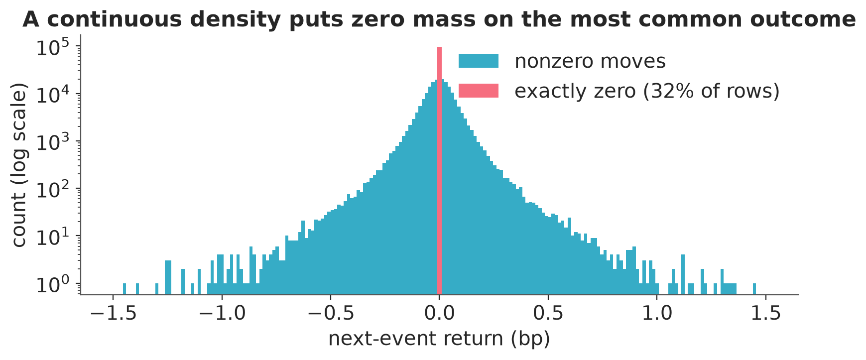
First, prices move on a discrete grid, so an exact-zero return is not a measure-zero event the way it is for a continuous variable: consecutive trades can and do leave the price where it was. A purely continuous likelihood puts zero probability mass on that outcome, whatever share of the rows it turns out to occupy. The fix is a hurdle: model whether the price moves separately from how far it moves given that it does.

Second, each row is a transition between consecutive observed events, not a fixed-duration return. So \(1 - \pi\) is the probability that the next event leaves the price unchanged, and \(\sigma\) is the Student-t scale conditional on a move. Neither is clock-time volatility: converting to a clock would additionally require a model of event arrival times [Engle and Russell, 1998].

\[\begin{split} \begin{aligned} m_i &\sim \text{Bernoulli}(\pi_i) \\ y_i \mid m_i = 1 &\sim \text{StudentT}(\nu,\ \mu_i,\ \sigma_i) \\ \operatorname{logit} \pi_i &= \kappa_0 + b^{(\kappa)}_s + B(h)^\top\!\left(c + b^{(\pi h)}_s\right) + \lambda_a a_i + \lambda_q q_i \\ \log \sigma_i &= \alpha_0 + b^{(\alpha)}_s + B(h)^\top\!\left(g + b^{(\sigma h)}_s\right) + (\beta_a + b^{(\beta a)}_s)\, a_i + \beta_q q_i \\ \mu_i &= \theta_d\, d_i + \theta_r\, \text{ylag}_i \end{aligned} \end{split}\]

where

• \(\kappa_0\) and \(\alpha_0\) are the global intercepts of the move probability and the log scale, and \(b^{(\kappa)}_s\), \(b^{(\alpha)}_s\) their per-symbol offsets;

• \(B(h)\) is the hour-of-day Fourier basis (four columns), \(c\) and \(g\) its global coefficients, and \(b^{(\pi h)}_s\), \(b^{(\sigma h)}_s\) the per-symbol deviations from them;

• \(\lambda_a\), \(\lambda_q\), \(\beta_a\), \(\beta_q\) are the covariate slopes, with \(b^{(\beta a)}_s\) a per-symbol slope on activity in the scale;

• \(\theta_d\), \(\theta_r\) place the conditional location on the trade sign and the last nonzero return;

• every \(b_s \sim \mathcal{N}(0, \tau)\) with its own \(\tau\), and \(\nu\) is shared.

The covariates are a simulated trade sign \(d_i\), a notional-like \(q_i\), an activity-like \(a_i\), and \(\text{ylag}_i\), the most recent previous nonzero return on that symbol. In the generator below they are drawn directly rather than engineered from a trade tape: only \(\text{ylag}\) is produced sequentially, so it is the one covariate that could not see the future, and \(q\) and \(a\) are standardized once over the whole sample. On a real archive both would instead be trailing statistics built causally from the tape and standardized with constants frozen on a burn-in window, a construction that is out of scope here and easy to get subtly wrong. \(B(h)\) is the first two sine/cosine harmonics of hour-of-day, a low-order version of the Fourier encoding of intraday periodicity in Andersen and Bollerslev [1997]; heavy-tailed Student-t noise for returns goes back at least to Bollerslev [1987]. All symbol effects \(b_s \sim \mathcal{N}(0, \tau)\) are partially pooled [Gelman and Hill, 2006], so a thin symbol is pulled toward the global intraday shape where its own data run out. They are parameterized centered, deliberately: the non-centered trick pays off when groups are data-poor, and the generator below gives every symbol at least several hundred rows. The degrees of freedom are shared across symbols, parameterized \(\nu = 1 + \operatorname{softplus}(\eta)\); the floor of 1 rather than 2 leaves the support open to tails too heavy to carry a finite variance. Under \(\eta \sim \mathcal{N}(5, 1)\) the prior puts only about \(4 \times 10^{-6}\) of its mass on \(\nu \le 2\), so this is a statement about support, not a serious prior belief in infinite variance. The estimand below is chosen so that the question does not arise at all.

The reported estimand is event-return dispersion on the event clock: \(\pi_{s,h}\) together with the conditional-move 90% half-width \(\sigma_{s,h} \cdot t^{-1}_{0.95}(\nu)\). A quantile is the safe choice here: it stays finite for any \(\nu > 0\), whereas a moment-based dispersion requires \(\nu > 2\), a constraint the model does not impose, even though the generator below happens to use \(\nu = 3.5\).

Synthetic data with known truth

This notebook neither ships nor downloads an exchange archive; the executed path uses a seeded synthetic generator: the schema an exchange archive would have after feature construction, a hurdle at exactly zero, heavy conditional tails, and twelve symbols whose row counts span two orders of magnitude, so the hierarchy has both data-rich and data-poor groups to work with. Because the truth is known, recovery is checkable. Every statement below about what the fit recovers is conditional on this generator; none of it is a measurement of any market.

n_symbols = 12
counts = np.array(
    [90_700, 55_000, 40_000, 30_000, 24_000, 19_000, 15_000, 11_000, 8_000, 4_600, 1_800, 900]
)
thin = [10, 11]  # the two symbols with the least data

truth = {
    "kappa0": np.log(0.7 / 0.3),  # logit(0.7): see the annotation below
    "c": np.array([0.25, -0.15, 0.10, 0.05]),
    "lambda_a": 0.35,
    "lambda_q": 0.20,
    "alpha0": np.log(0.05),  # conditional-move scale, in basis points
    "g": np.array([0.20, -0.12, 0.08, 0.04]),
    "beta_a": 0.18,
    "beta_q": 0.12,
    "theta_d": 0.02,
    "theta_r": 0.25,
    "nu": 3.5,
}


def standardize(x, axis=0):
    return (x - x.mean(axis=axis, keepdims=True)) / x.std(axis=axis, keepdims=True)


z_truth = {
    "z_k": standardize(rng.standard_normal(n_symbols)),
    "z_ph": standardize(rng.standard_normal((n_symbols, 4))),
    "z_al": standardize(rng.standard_normal(n_symbols)),
    "z_sh": standardize(rng.standard_normal((n_symbols, 4))),
    "z_ba": standardize(rng.standard_normal(n_symbols)),
}

def hour_basis(hour):
    w = 2 * np.pi * np.asarray(hour, dtype=float) / 24.0
    return np.column_stack([np.sin(w), np.cos(w), np.sin(2 * w), np.cos(2 * w)])


sym = np.repeat(np.arange(n_symbols), counts)
n = len(sym)
hour = rng.integers(0, 24, size=n)
d = rng.choice([-1.0, 1.0], size=n)
a = standardize(rng.standard_normal(n))  # trailing activity (already standardized)
q = standardize(0.3 * a + np.sqrt(1 - 0.3**2) * rng.standard_normal(n))

B = hour_basis(hour)
logit_pi = (
    truth["kappa0"]
    + 0.30 * z_truth["z_k"][sym]
    + B @ truth["c"]
    + (B * (0.15 * z_truth["z_ph"][sym])).sum(1)
    + truth["lambda_a"] * a
    + truth["lambda_q"] * q
)
log_sigma = (
    truth["alpha0"]
    + 0.35 * z_truth["z_al"][sym]
    + B @ truth["g"]
    + (B * (0.12 * z_truth["z_sh"][sym])).sum(1)
    + (truth["beta_a"] + 0.10 * z_truth["z_ba"][sym]) * a
    + truth["beta_q"] * q
)

m = (rng.random(n) < 1 / (1 + np.exp(-logit_pi))).astype(np.int8)
t_draw = rng.standard_t(truth["nu"], size=n)

# sequential generation per symbol so ylag feeds back causally
y = np.zeros(n)
ylag = np.zeros(n)
sigma = np.exp(log_sigma)
for s in range(n_symbols):
    idx = np.flatnonzero(sym == s)
    last = 0.0
    for i in idx:
        ylag[i] = last
        if m[i]:
            y[i] = truth["theta_d"] * d[i] + truth["theta_r"] * last + sigma[i] * t_draw[i]
            last = y[i]

print(
    f"{n:,} rows, zero-move share {(m == 0).mean():.1%}, "
    f"median nonzero |y| {np.median(np.abs(y[m == 1])):.3f} bp, "
    f"corr(a, q) {np.corrcoef(a, q)[0, 1]:.2f}"
)

300,000 rows, zero-move share 32.1%, median nonzero |y| 0.041 bp, corr(a, q) 0.30

The constants above are settings, not measurements. Read them as the specification of the simulator:

• kappa0 = \(\operatorname{logit}(0.7)\). If every other term in the logit were zero, the move probability would be 0.7. The harmonics, the covariates and the symbol effects all shift it, so the realized zero share is the number printed above, not \(30\%\) by construction.

• theta_r \(= 0.25\) imposes positive first-order dependence in the conditional location: the next move is generated partly from the previous nonzero one. It is a synthetic dependence parameter; note that the classical bid–ask bounce of Roll [1984] runs the other way, inducing negative serial dependence, which this generator does not encode.

• theta_d \(= 0.02\) is the coefficient on the simulated trade sign: holding everything else fixed, sign \(+1\) versus \(-1\) differs by 0.04 bp in conditional location.

• \(a\) and \(q\) are constructed with a target correlation of 0.3 rather than orthogonally, so the fit faces mildly collinear covariates instead of a textbook design; the realized sample correlation is in the printout above.

• ylag is generated per symbol in sequence, so row \(i\) sees only the most recent previously generated nonzero move. That discipline applies to the lag construction; the standardization of \(a\) and \(q\) still uses full-sample constants, an offline simplification kept for readability.

With that in mind, here is the feature that forces the hurdle:

fig, ax = plt.subplots(figsize=(8, 3.5), layout="constrained")
moves = y[m == 1]
ax.hist(moves, bins=201, range=(-1.5, 1.5), log=True, color="C0", label="nonzero moves")
ax.bar(
    [0.0],
    [(m == 0).sum()],
    width=0.02,
    color="C1",
    label=f"exactly zero ({(m == 0).mean():.0%} of rows)",
)
ax.set_xlabel("next-event return (bp)")
ax.set_ylabel("count (log scale)")
ax.set_title("A continuous density puts zero mass on the most common outcome")
ax.legend();

The on-disk global shuffle

Streaming ordered data has one trap that is easy to miss. A bounded runtime shuffle buffer only block-shuffles a strongly ordered stream: with tick data sorted by symbol and time, early optimization steps would only ever see early dates and the first symbols, and an early stopping decision would be biased by construction. The fix is to shuffle once, globally, on disk when the archive is written: every row gets a deterministic hash key, rows are scattered across shards by that key, and each shard is sorted by it. After that, sequential reads follow one fixed, data-independent permutation. It is pseudo-random (a hash of the row index, nothing from the row itself) and replayed identically each epoch, so this is single-shuffle stochastic gradient descent rather than fresh per-step subsampling. The loader can then run with shuffle=False, without a copy through the shuffle buffer.

data_dir = tempfile.mkdtemp(prefix="ticks_")
table = pa.table(
    {
        "y_bp": y.astype(np.float32),
        "m": m,
        "d": d.astype(np.int8),
        "q_std": q.astype(np.float32),
        "a_std": a.astype(np.float32),
        "ylag_bp": ylag.astype(np.float32),
        "hour": hour.astype(np.int8),
        "sym": sym.astype(np.int16),
    }
)


def splitmix64(x):
    x = (x + np.uint64(0x9E3779B97F4A7C15)) & np.uint64(0xFFFFFFFFFFFFFFFF)
    x = ((x ^ (x >> np.uint64(30))) * np.uint64(0xBF58476D1CE4E5B9)) & np.uint64(0xFFFFFFFFFFFFFFFF)
    x = ((x ^ (x >> np.uint64(27))) * np.uint64(0x94D049BB133111EB)) & np.uint64(0xFFFFFFFFFFFFFFFF)
    return x ^ (x >> np.uint64(31))


key = splitmix64(np.arange(n, dtype=np.uint64))
order = np.argsort(key, kind="stable")
n_shards, BATCH = 10, 1_000
# Row groups are the loader's batches on the shuffle=False path, so the geometry is
# chosen to divide exactly: 10 shards x 30,000 rows, 30 groups of 1,000 each.
assert n % n_shards == 0 and (n // n_shards) % BATCH == 0
for i in range(n_shards):
    part = table.take(order[i::n_shards])
    pq.write_table(part, os.path.join(data_dir, f"shard_{i:03d}.parquet"), row_group_size=BATCH)

# the head of every shard has to mix hours and symbols already; check all of them
for i in range(n_shards):
    head = pq.read_table(os.path.join(data_dir, f"shard_{i:03d}.parquet")).slice(0, 10_000)
    assert len(np.unique(head["hour"])) == 24
    assert len(np.unique(head["sym"])) == n_symbols
print(f"first 10k rows of every shard cover all 24 hours and all {n_symbols} symbols")

first 10k rows of every shard cover all 24 hours and all 12 symbols

The assertion is the one to keep: the head of every shard must already mix every hour and every symbol, checked rather than assumed.

This cell is a small-scale stand-in for the real extract-transform-load step: it builds the whole table, the whole key array and the whole permutation in memory, which is exactly what one cannot do once the data stops fitting. The inference that follows really does read from disk; the preprocessing above does not. An out-of-core design with the same properties is two passes: assign each row to a shard from its hash key, appending row groups of bounded size, then sort each shard by key independently, so no step holds more than one shard. That yields a different permutation from the rank-based split used here (shard sizes come out approximately rather than exactly equal), with the same guarantee that no shard’s order depends on anything in the rows.

So that the fit really does run against disk rather than against arrays still resident from the generator, the row-scale objects are released first:

del table, part, head, key, order, y, m, d, q, a, ylag, sym, hour, B, moves
del logit_pi, log_sigma, t_draw, sigma
gc.collect()
print("row-scale generator arrays released; the fit reads from", os.path.basename(data_dir))

row-scale generator arrays released; the fit reads from ticks_nihg_s5h

Streaming the model

With shuffle=False the DataLoader passes source blocks through verbatim, one block per Parquet row group, in a frozen column order. That is why the shards above were written with row_group_size equal to the batch size, and why the row counts were chosen to divide exactly. On this path the loader hands you the row groups it finds. A ragged geometry therefore gives ragged batches; len(loader) (which is total_size // batch_size) stops matching the number of blocks an epoch yields; and the recorded loss picks up a deterministic sawtooth that has nothing to do with convergence (the fitting section explains why the recorded value scales with the block size). The model reads one pm.Data placeholder; everything derived (the Fourier basis, the integer symbol index) is computed inside the graph, so advancing the stream is a single set_value per step.

columns = ["y_bp", "m", "d", "q_std", "a_std", "ylag_bp", "hour", "sym"]
loader = DataLoader(
    parquet_source(data_dir, columns=columns),
    batch_size=BATCH,
    shuffle=False,  # the shards are already globally shuffled on disk
    total_size="auto",
)

# Count one epoch rather than inferring it. With a divisible geometry every block
# is the same size, so the count and len(loader) agree — which is what the rest of
# the notebook relies on.
block_rows = [b.shape[0] for b in loader]
steps_per_epoch = len(block_rows)
assert set(block_rows) == {BATCH}
assert sum(block_rows) == loader.total_size == n == steps_per_epoch * BATCH
assert len(loader) == steps_per_epoch
print(
    f"N = {loader.total_size:,} rows -> {steps_per_epoch} blocks of {BATCH} per epoch,\n"
    f"conserving {sum(block_rows):,} rows; len(loader) = {len(loader)}"
)

N = 300,000 rows -> 300 blocks of 1000 per epoch,
conserving 300,000 rows; len(loader) = 300

That assertion pins down two things. First, nothing is dropped: verbatim pass-through streams every row exactly once per epoch. (Ragged geometry would still lose nothing, since PyMC reads b from the batch actually installed and a short block is weighted up by its own size, but it would cost the clean diagnostics below, which is why the shards divide.) Only the shuffle-buffer path drops a trailing partial batch, and this notebook never uses it.

Second, this is where the Gate 1 distinction bites: the batch at step \(t\) is a deterministic function of \(t\), so what follows is single-shuffle, cyclic finite-sum optimization, the arrangement the epoch-scale diagnostics later in the notebook exploit and the reason the fit has to be summarized with some care before anything is read off it.

def build_model(symbols, batch_init, total_size):
    coords = {"symbol": list(symbols), "harmonic": ["sin1", "cos1", "sin2", "cos2"]}
    with pm.Model(coords=coords) as model:
        batch = pm.Data("batch", batch_init)
        y_ = batch[:, 0]
        d_ = batch[:, 2]
        q_ = batch[:, 3]
        a_ = batch[:, 4]
        ylag_ = batch[:, 5]
        w = 2.0 * np.pi * batch[:, 6] / 24.0
        B_ = pt.stack([pt.sin(w), pt.cos(w), pt.sin(2 * w), pt.cos(2 * w)], axis=1)
        sym_ = pt.cast(batch[:, 7], "int32")

        kappa0 = pm.Normal("kappa0", 0.0, 5.0)
        c = pm.Normal("c", 0.0, 0.5, dims="harmonic")
        lambda_a = pm.Normal("lambda_a", 0.0, 0.5)
        lambda_q = pm.Normal("lambda_q", 0.0, 0.5)

        alpha0 = pm.Normal("alpha0", 0.0, 5.0)
        g = pm.Normal("g", 0.0, 0.3, dims="harmonic")
        beta_a = pm.Normal("beta_a", 0.0, 0.3)
        beta_q = pm.Normal("beta_q", 0.0, 0.3)

        theta_d = pm.Normal("theta_d", 0.0, 0.25)
        theta_r = pm.Normal("theta_r", 0.0, 0.25)

        tau_k, tau_ph, tau_al, tau_sh, tau_ba = (
            pm.LogNormal(name, 0.0, 1.5)
            for name in ["tau_k", "tau_ph", "tau_al", "tau_sh", "tau_ba"]
        )
        b_k = pm.Normal("b_k", 0.0, tau_k, dims="symbol")
        b_ph = pm.Normal("b_ph", 0.0, tau_ph, dims=("symbol", "harmonic"))
        b_al = pm.Normal("b_al", 0.0, tau_al, dims="symbol")
        b_sh = pm.Normal("b_sh", 0.0, tau_sh, dims=("symbol", "harmonic"))
        b_ba = pm.Normal("b_ba", 0.0, tau_ba, dims="symbol")

        eta = pm.Normal("eta", 5.0, 1.0)
        nu = pm.Deterministic("nu", 1.0 + pt.softplus(eta))

        logit_pi = (
            kappa0
            + b_k[sym_]
            + (B_ * (c + b_ph[sym_])).sum(axis=-1)
            + lambda_a * a_
            + lambda_q * q_
        )
        log_sigma = (
            alpha0
            + b_al[sym_]
            + (B_ * (g + b_sh[sym_])).sum(axis=-1)
            + (beta_a + b_ba[sym_]) * a_
            + beta_q * q_
        )
        mu = theta_d * d_ + theta_r * ylag_

        def hurdle_logp(value, logit_pi, mu, log_sigma, nu):
            # one coherent mixed distribution: an atom at exactly zero plus a
            # Student-t density off zero — the move indicator is value != 0,
            # never a separate parameter, so logp and random describe the SAME law
            sigma = pt.exp(log_sigma)
            t_ll = (
                pt.gammaln((nu + 1.0) / 2.0)
                - pt.gammaln(nu / 2.0)
                - 0.5 * pt.log(nu * np.pi)
                - log_sigma
                - (nu + 1.0) / 2.0 * pt.log1p(((value - mu) / sigma) ** 2 / nu)
            )
            moved = pt.neq(value, 0.0)
            return pt.where(moved, -pt.softplus(-logit_pi) + t_ll, -pt.softplus(logit_pi))

        def hurdle_random(logit_pi, mu, log_sigma, nu, rng=None, size=None):
            # simulate the same law: first whether the price moves, then how far
            pi = 1.0 / (1.0 + np.exp(-logit_pi))
            move = rng.random(size=size) < pi
            draw = mu + np.exp(log_sigma) * rng.standard_t(nu, size=size)
            return np.where(move, draw, 0.0)

        pm.CustomDist(
            "y_obs",
            logit_pi,
            mu,
            log_sigma,
            nu,
            logp=hurdle_logp,
            random=hurdle_random,
            observed=y_,
            total_size=total_size,
        )
    return model

Two implementation notes. The likelihood is a CustomDist with a logp, not a pm.Potential: CustomDist gives the term observed random-variable semantics, which is what makes PyMC’s own total_size minibatch rescaling apply. And the hurdle’s two logs are written with softplus, \(\log \pi = -\operatorname{softplus}(-x)\) and \(\log(1-\pi) = -\operatorname{softplus}(x)\), which is exact and stable at both tails. The exact float comparison value != 0 is safe here because the zeros are structural: the generator writes an exact 0.0 when the hurdle says the price did not move, and every nonzero draw is many orders of magnitude above the float32 subnormal range. On real data the same comparison is safe as long as returns are computed so that “no move” produces an exact zero rather than a rounding artifact; check that once, in the feature code.

model = build_model(
    [f"SYM{i:02d}" for i in range(n_symbols)], next(iter(loader)), loader.total_size
)
pm.model_to_graphviz(model)

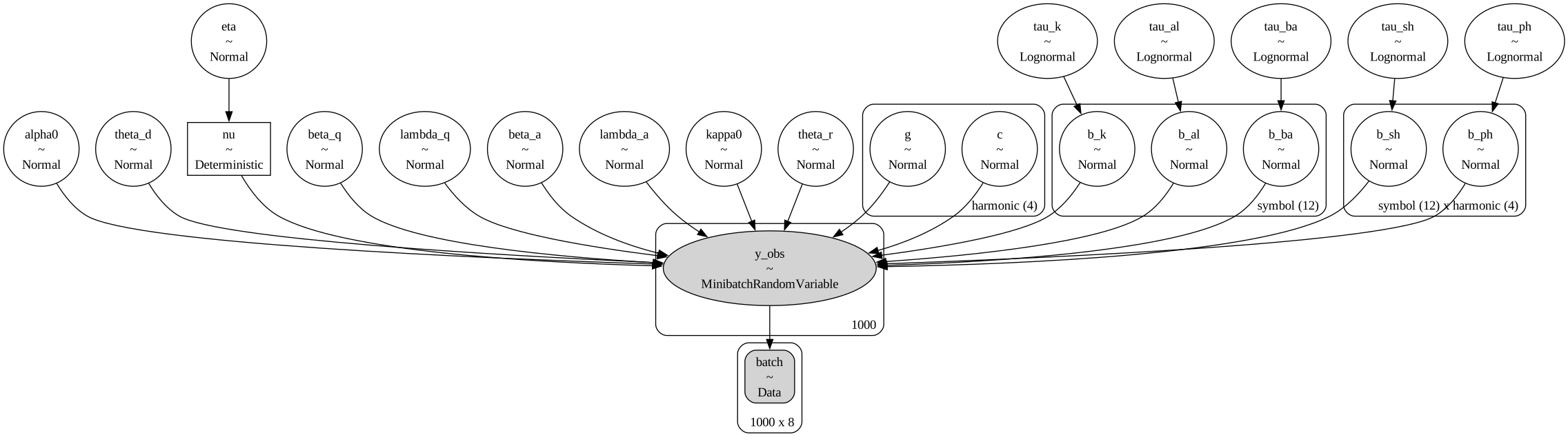
The plate diagram is an inventory rather than a picture of the two links: five partially pooled effect families on the symbol plate, one shared tail parameter, and a single observed node whose batch dimension is whatever the placeholder currently holds. The two linear predictors live inside the likelihood’s logp and are not separate nodes; the equations above are where that structure is visible.

The loop below is the whole streaming adapter: a pm.fit callback that pushes the next block into the placeholder after each step; the twenty lines here are the minimal version a notebook can own (a library wrapper for the same lifecycle is listed at the end).

class StreamAdvance:
    """pm.fit callback: put the next minibatch into the placeholder after each step."""

    def __init__(self, model, loader):
        self._shared = model["batch"]
        self._stream = self._endless(loader)

    @staticmethod
    def _endless(loader):
        while True:
            yield from loader

    def prime(self):
        self._shared.set_value(next(self._stream), borrow=True)

    def __call__(self, approx, losses, i):
        self._shared.set_value(next(self._stream), borrow=True)


class ParamTrace:
    """pm.fit callback: record the variational parameters after every step."""

    def __init__(self):
        self.mu, self.rho = [], []

    def __call__(self, approx, losses, i):
        mu, rho = approx.params
        self.mu.append(mu.get_value())
        self.rho.append(rho.get_value())


stream = StreamAdvance(model, loader)
stream.prime()
tail = ParamTrace()

with model:
    advi = pm.ADVI(random_seed=RANDOM_SEED)
advi.fit(6_000, obj_optimizer=pm.adam(learning_rate=0.02), callbacks=[stream], progressbar=False)
approx = advi.fit(
    2_400,
    obj_optimizer=pm.adam(learning_rate=0.005),
    callbacks=[stream, tail],
    progressbar=False,
)

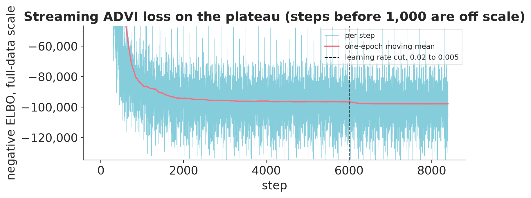
The fit is mean-field ADVI [Kucukelbir et al., 2015] driven by Adam. The learning rate is cut once, at step 6,000. A constant step size that is comfortable early is too large near the optimum, where it keeps the variational mean bouncing instead of settling; dropping it once the descent has flattened is the cheapest fix. The effect does not show up in the width of the loss band below: the band is dominated by batch-composition noise (the stopping section shows it all but vanishing at epoch-aligned horizons), and the printed spread is the same on both sides of the change. It shows up in the level, as the printed one-epoch means either side of the cut, and in the parameter trace examined after the fit.

Before plotting it, one property of approx.hist that is easy to get wrong and that changes what the numbers mean. PyMC normalizes the minibatch objective twice: the observed log-probability is scaled up by \(N/b\) so the gradient targets the full-data model, and then the variational objective is divided by that same constant, because scale_cost_to_minibatch is on by default. What gets recorded per step is therefore

\[ F_t = -\sum_{i \in \mathcal{B}_t} \mathbb{E}_q\left[\log p(y_i \mid \theta)\right] + \frac{b}{N}\,\mathrm{KL}(q \Vert p), \]

where \(\mathcal{B}_t\) is the set of rows in the batch at step \(t\), \(b\) its size, \(N\) the total row count (loader.total_size), \(\theta\) the parameters, \(q\) the variational approximation, \(p\) the prior, and \(\mathrm{KL}\) the Kullback–Leibler divergence. This lives on the scale of one batch, not of the full dataset, and would move mechanically with \(b\) if the blocks were ragged. Multiplying by \(N/b\) puts it back on the full-data scale of the negative evidence lower bound (ELBO), and with equal blocks that is one constant:

ELBO_SCALE = loader.total_size / BATCH  # undo PyMC's scale_cost_to_minibatch
loss = np.asarray(approx.hist, dtype=float) * ELBO_SCALE

epoch_mean = np.convolve(loss, np.ones(steps_per_epoch) / steps_per_epoch, mode="valid")

fig, ax = plt.subplots(figsize=(8, 3.2), layout="constrained")
ax.plot(loss, lw=0.5, alpha=0.6, label="per step")
ax.plot(
    np.arange(steps_per_epoch - 1, len(loss)),
    epoch_mean,
    color="C1",
    lw=1.5,
    label="one-epoch moving mean",
)
ax.axvline(6_000, color="k", ls="--", lw=1, label="learning rate cut, 0.02 to 0.005")
# clip to the plateau: the first few hundred steps are orders of magnitude higher
plateau = loss[1_000:]
ax.set_ylim(np.quantile(plateau, 0.001), np.quantile(plateau, 0.999))
ax.yaxis.set_major_formatter(StrMethodFormatter("{x:,.0f}"))
ax.set_xlabel("step")
ax.set_ylabel("negative ELBO, full-data scale")
ax.set_title("Streaming ADVI loss on the plateau (steps before 1,000 are off scale)")
ax.legend(loc="upper right", fontsize=9, frameon=True)
before, after = loss[6_000 - 2 * steps_per_epoch : 6_000], loss[6_000 : 6_000 + 2 * steps_per_epoch]
print(
    "recorded loss over the two passes either side of the cut:\n"
    f"  spread (sd): {before.std():,.0f} before, {after.std():,.0f} after\n"
    f"  level (mean): {before.mean():,.0f} before, {after.mean():,.0f} after"
);

recorded loss over the two passes either side of the cut:
  spread (sd): 13,192 before, 13,093 after
  level (mean): -96,528 before, -97,746 after

The last iterate is not the answer

Before reading a single parameter off this fit, one property of the replay has to be dealt with. The batch at step \(t\) is a deterministic function of \(t\) with period one epoch, so the data term of every stochastic gradient repeats with that period. The parameters and the Monte Carlo draw do not, so the realized gradients are not literally periodic, but the iterate inherits a component locked to the replay order. Two measurements separate that component from genuine progress: compare the same phase in consecutive epochs, and look at the spread within a single epoch.

mu_t = np.asarray(tail.mu)
sd_unc = approx.std.eval()  # variational sd in the unconstrained space, before averaging
ends = mu_t[steps_per_epoch - 1 :: steps_per_epoch]  # same phase, one epoch apart
step = np.abs(np.diff(ends, axis=0)) / sd_unc  # (7 epoch pairs, 154 coordinates)
last = mu_t[-steps_per_epoch:]
swing = (last.max(0) - last.min(0)) / sd_unc
print(
    "same phase, epoch to epoch, max over coordinates per pair:\n  "
    + " ".join(f"{v:.2f}" for v in step.max(1))
    + f"\n  median over coordinates, last pair: {np.median(step[-1]):.2f} sd"
    f"\nwithin the last epoch: median {np.median(swing):.2f}, max {swing.max():.1f} sd"
)

same phase, epoch to epoch, max over coordinates per pair:
  6.37 2.93 2.59 0.75 1.39 1.45 0.58
  median over coordinates, last pair: 0.11 sd
within the last epoch: median 4.31, max 41.2 sd

Between the same phase of consecutive epochs the largest movement decays from about six posterior widths in the first pair to about half a width in the last, and the median coordinate moves a tenth of a width per pass; within a single epoch the same coordinates swing by multiples of their width. So the optimizer is not converging to a point. It is orbiting one, on a cycle locked to the order the rows are replayed in, and most of where the last iterate sits is the phase of that orbit at the step the budget ran out.

The number you would report therefore depends on where you stop, so the fit is summarized by averaging the variational parameters over the final whole pass. To the extent the order-locked component repeats from one pass to the next, a window of exactly one pass averages it out (which is why the step budget above is a whole number of epochs), and a window that is not a whole number of passes leaves a residual of the order of one swing divided by the window length. This is Polyak–Ruppert averaging [Polyak and Juditsky, 1992]. What the average does not remove is the slow drift the first line still shows: a tenth of a width per pass in the median, and much more along the directions the recovery table is about to single out.

rho_t = np.asarray(tail.rho)
approx.params[0].set_value(mu_t[-steps_per_epoch:].mean(0))
approx.params[1].set_value(rho_t[-steps_per_epoch:].mean(0))
print(f"variational parameters averaged over the final {steps_per_epoch} steps (one epoch)")

variational parameters averaged over the final 300 steps (one epoch)

Everything below reads from that averaged approximation.

Did it recover the truth?

idata = approx.sample(2_000, random_seed=RANDOM_SEED)
post = idata.posterior

scalar_params = [
    "kappa0",
    "alpha0",
    "lambda_a",
    "lambda_q",
    "beta_a",
    "beta_q",
    "theta_d",
    "theta_r",
    "nu",
]
rows = {name: [float(post[name].mean()), float(post[name].std())] for name in scalar_params}
# the intercepts share a ridge with their group means; only the sums are identified
for intercept, b in [("kappa0", "b_k"), ("alpha0", "b_al"), ("beta_a", "b_ba")]:
    s = post[intercept] + post[b].mean("symbol")
    rows[f"{intercept} + mean({b})"] = [float(s.mean()), float(s.std())]
recovery = pd.DataFrame(rows, index=["mean", "sd"]).T
recovery["truth"] = [truth[p] for p in scalar_params] + [
    truth["kappa0"],
    truth["alpha0"],
    truth["beta_a"],
]
recovery["abs_error"] = (recovery["mean"] - recovery["truth"]).abs()
recovery["z"] = (recovery["mean"] - recovery["truth"]) / recovery["sd"]
recovery.round(4)

	mean	sd	truth	abs_error	z
kappa0	0.5336	0.0048	0.8473	0.3137	-65.2181
alpha0	-1.7012	0.0034	-2.9957	1.2946	378.5027
lambda_a	0.3517	0.0053	0.3500	0.0017	0.3298
lambda_q	0.2065	0.0056	0.2000	0.0065	1.1587
beta_a	0.1624	0.0036	0.1800	0.0176	-4.8789
beta_q	0.1223	0.0031	0.1200	0.0023	0.7391
theta_d	0.0200	0.0002	0.0200	0.0000	-0.0473
theta_r	0.2500	0.0019	0.2500	0.0000	0.0151
nu	3.5097	0.0230	3.5000	0.0097	0.4224
kappa0 + mean(b_k)	0.8495	0.0096	0.8473	0.0022	0.2253
alpha0 + mean(b_al)	-2.9948	0.0064	-2.9957	0.0009	0.1427
beta_a + mean(b_ba)	0.1813	0.0057	0.1800	0.0013	0.2236

# Is the table a property of the problem or of one optimizer trajectory? Three
# more readings of the same data and budget: the notebook's own last iterate
# before averaging; a refit with a different optimizer seed on the same replay
# order; and a refit on a different on-disk order — the replay order is the one
# ingredient the orbit story is about, so it is the one worth varying.
raw_splits = ["kappa0", "alpha0", "beta_a"]
identified = [name for name in recovery.index if name not in raw_splits]


def summarize(post_):
    """Posterior mean and sd of every row the recovery table reports."""
    out = {name: (float(post_[name].mean()), float(post_[name].std())) for name in scalar_params}
    for intercept, b in [("kappa0", "b_k"), ("alpha0", "b_al"), ("beta_a", "b_ba")]:
        total = post_[intercept] + post_[b].mean("symbol")
        out[f"{intercept} + mean({b})"] = (float(total.mean()), float(total.std()))
    return pd.DataFrame(out, index=["mean", "sd"]).T


def reshuffle(src_dir, salt):
    """A second on-disk order: re-key the already-shuffled rows with a different salt."""
    dst_dir = tempfile.mkdtemp(prefix="ticks_reorder_")
    full = pa.concat_tables(
        [pq.read_table(os.path.join(src_dir, f)) for f in sorted(os.listdir(src_dir))]
    )
    order2 = np.argsort(
        splitmix64(np.arange(full.num_rows, dtype=np.uint64) + np.uint64(salt)), kind="stable"
    )
    for i in range(n_shards):
        pq.write_table(
            full.take(order2[i::n_shards]),
            os.path.join(dst_dir, f"shard_{i:03d}.parquet"),
            row_group_size=BATCH,
        )
    return dst_dir


def refit(seed, data_loader):
    stream_s, tail_s = StreamAdvance(model, data_loader), ParamTrace()
    stream_s.prime()
    with model:
        advi_s = pm.ADVI(random_seed=seed)
    advi_s.fit(
        6_000, obj_optimizer=pm.adam(learning_rate=0.02), callbacks=[stream_s], progressbar=False
    )
    approx_s = advi_s.fit(
        2_400,
        obj_optimizer=pm.adam(learning_rate=0.005),
        callbacks=[stream_s, tail_s],
        progressbar=False,
    )
    approx_s.params[0].set_value(np.asarray(tail_s.mu)[-steps_per_epoch:].mean(0))
    approx_s.params[1].set_value(np.asarray(tail_s.rho)[-steps_per_epoch:].mean(0))
    return summarize(approx_s.sample(2_000, random_seed=seed).posterior)


approx.params[0].set_value(mu_t[-1])
approx.params[1].set_value(rho_t[-1])
last_iterate = summarize(approx.sample(2_000, random_seed=RANDOM_SEED).posterior)
approx.params[0].set_value(mu_t[-steps_per_epoch:].mean(0))
approx.params[1].set_value(rho_t[-steps_per_epoch:].mean(0))

other_dir = reshuffle(data_dir, salt=1)
other_loader = DataLoader(
    parquet_source(other_dir, columns=columns), batch_size=BATCH, shuffle=False, total_size="auto"
)
readings = {
    "last iterate": last_iterate,
    "seed 0": recovery[["mean", "sd"]],
    "seed 1, same order": refit(RANDOM_SEED + 1, loader),
    "seed 2, other order": refit(RANDOM_SEED + 2, other_loader),
}
tru = recovery.loc[identified, "truth"]
z_own = {
    k: ((v.loc[identified, "mean"] - tru) / v.loc[identified, "sd"]).abs().max()
    for k, v in readings.items()
}
means = pd.DataFrame(
    {k: v.loc[identified, "mean"] for k, v in readings.items() if k != "last iterate"}
)
spread = means.std(axis=1) / recovery.loc[identified, "sd"]
print(
    "identified rows, max |z| against the truth, each fit in its own posterior sd:\n  "
    + "\n  ".join(f"{k}: {v:.2f}" for k, v in z_own.items())
    + "\nspread of the mean across the three tail-averaged fits, in seed-0 sd:"
    f"\n  median {spread.median():.2f}, max {spread.max():.2f}"
)

identified rows, max |z| against the truth, each fit in its own posterior sd:
  last iterate: 3.42
  seed 0: 1.16
  seed 1, same order: 1.14
  seed 2, other order: 1.13
spread of the mean across the three tail-averaged fits, in seed-0 sd:
  median 0.08, max 0.10

The table is a selection, the scalar globals and the three identified sums, and the figure after it checks one of the five symbol-effect families; that, plus the two curves for one symbol further down, is the extent of the recovery evidence here. Read the table bottom-up. The raw intercepts look off by 0.3 and 1.3, but a global coefficient and the mean of its group effects are only jointly pinned by the likelihood, which is exactly flat along \((\alpha_0 + d,\ b^{(\alpha)} - d)\). What tilts that direction at all is the hierarchical prior: shifting every symbol effect by \(d\) costs \(\sum_s (b_s - d)^2 / 2\tau^2\), which is minimized when the effects average to zero, and the generator standardized them to average exactly zero, so the prior points the split at the generating value. Conditional on everything else, that cost is a Gaussian in \(d\) with standard deviation \(\tau/\sqrt{12}\), a tenth for \(\tau\) near the generator’s \(0.35\), which is the scale of uncertainty the split actually carries. The same translation ridge exists for every global-coefficient/group-effect pair in this model (including the vector pairs \(c\)/\(b^{(\pi h)}\) and \(g\)/\(b^{(\sigma h)}\), whose sums the table omits).

Two things follow, and the table shows both. Along a direction that flat, a gradient optimizer crawls: 8,400 steps have carried alpha0 to \(-1.70\) on its way to \(-3.00\). To see that it is still traveling, warm-start a fresh optimizer at the last iterate and give it sixty more passes at the same learning rate:

# Continue from the last iterate on a fresh optimizer, so `approx` and its loss
# history above are left exactly as they were.
with model:
    advi_more = pm.ADVI(random_seed=RANDOM_SEED)
advi_more.approx.params[0].set_value(mu_t[-1])
advi_more.approx.params[1].set_value(rho_t[-1])
stream_more = StreamAdvance(model, loader)
stream_more.prime()
where = {name: approx.ordering[name][1].start for name in ["kappa0", "alpha0"]}
path = [[mu_t[-1][where["kappa0"]], mu_t[-1][where["alpha0"]]]]  # +0 passes


class EpochMeans:
    def __call__(self, approx_, losses, i):
        if i % steps_per_epoch == 0:
            mu_now = approx_.params[0].get_value()
            path.append([mu_now[where["kappa0"]], mu_now[where["alpha0"]]])


advi_more.fit(
    60 * steps_per_epoch,
    obj_optimizer=pm.adam(learning_rate=0.005),
    callbacks=[stream_more, EpochMeans()],
    progressbar=False,
)
path = np.asarray(path)
more_loss = np.asarray(advi_more.hist) * ELBO_SCALE
print(
    "after +0 / +30 / +60 passes\n"
    f"  kappa0: {' / '.join(f'{v:.3f}' for v in path[[0, 30, 60], 0])} (generating {truth['kappa0']:.3f})\n"
    f"  alpha0: {' / '.join(f'{v:.3f}' for v in path[[0, 30, 60], 1])} (generating {truth['alpha0']:.3f})\n"
    "  loss per pass over those 60: "
    f"{(more_loss[-steps_per_epoch:].mean() - more_loss[:steps_per_epoch].mean()) / 59:+.2f} nats"
)

after +0 / +30 / +60 passes
  kappa0: 0.533 / 0.579 / 0.628 (generating 0.847)
  alpha0: -1.702 / -1.711 / -1.722 (generating -2.996)
  loss per pass over those 60: -0.37 nats

The ridge coordinates keep moving toward their generating values, at a rate the loss barely registers. The raw split rows are a fit still traveling along a nearly flat direction, not an ambiguity in the model. And their reported widths, a few thousandths, are the mean-field conditional width across the ridge, not the tenth just computed along it: mean-field has no correlation to spend, so it reports the narrow direction as if it were the wide one, which is why alpha0 reads \(z = 379\). Both are reasons a sum-to-zero constraint on the symbol effects is the standard reparameterization when the split itself matters: it removes the direction instead of asking the optimizer to find its way along it.

The identified rows are a different story. Every row the table reports that is pinned by the likelihood, the three sums and the six standalone coefficients, lands inside \(1.2\) posterior standard deviations of its generating value, and seven of those nine are inside \(0.5\). The replicate cell puts that in context from two directions. Read from the last iterate instead of the tail average, the same rows ran to \(3.4\); that difference was the orbit, not the estimate. And on two refits, one with a different optimizer seed on the same replay order and one on a different on-disk order altogether, the identified rows land in the same range, each fit judged in its own posterior width, with the spread of the means across the three tail-averaged fits about a tenth of the reported width. That is the replication check, and what it buys is limited. Material disagreement between fits would have been enough to withhold any claim about a width; agreement only removes the instability warning. It does not validate calibration. The widths here are those of a mean-field approximation, and z-scores this small on one dataset are consistent with widths that are somewhat too narrow, somewhat too wide, or right; sizing that needs many simulated datasets, and this notebook fits one.

The more interesting check is hierarchical: what happened to the per-symbol effects of the two symbols with 1,800 and 900 rows?

# plot the identified CONTRAST b - mean(b): the table above showed the absolute
# level belongs to a ridge with the intercept, so comparing raw b to raw truth
# would only display the arbitrary level split. Hand-rolled rather than
# az.plot_forest because the display is bespoke: truth overlay + thin shading.
bc = post["b_al"] - post["b_al"].mean("symbol")
b_mean = bc.mean(("chain", "draw")).values
b_sd = bc.std(("chain", "draw")).values
b_truth = 0.35 * z_truth["z_al"]  # the generator's scale times its z draws
b_truth = b_truth - b_truth.mean()

fig, ax = plt.subplots(figsize=(8, 3.5), layout="constrained")
x = np.arange(n_symbols)
ax.errorbar(
    x,
    b_mean,
    yerr=2 * b_sd,
    fmt="o",
    color="C0",
    capsize=3,
    label="mean ± 2 posterior sd (mean-field)",
)
ax.scatter(x, b_truth, marker="x", color="C1", s=60, zorder=3, label="truth")
for t in thin:
    ax.axvspan(t - 0.4, t + 0.4, color="C3", alpha=0.12)
ax.set_xticks(x)
ax.set_xticklabels([f"S{i}" for i in x])
ax.set_xlabel("symbol (shaded = thin: 1,800 and 900 rows)")
ax.set_ylabel(r"$b^{(\alpha)}_s - \bar{b}^{(\alpha)}$")
ax.set_title("Symbol effects against the generating values (thin symbols shaded)")
ax.legend()

order = np.argsort(-b_sd)
print(
    "posterior sd of the contrast, widest first:\n  "
    + ", ".join(f"S{i:02d} {b_sd[i]:.3f} ({counts[i]:,} rows)" for i in order[:3])
    + f"\n  ... narrowest S{order[-1]:02d} {b_sd[order[-1]]:.3f} ({counts[order[-1]]:,} rows)"
)

posterior sd of the contrast, widest first:
  S11 0.044 (900 rows), S10 0.023 (1,800 rows), S09 0.019 (4,600 rows)
  ... narrowest S00 0.007 (90,700 rows)

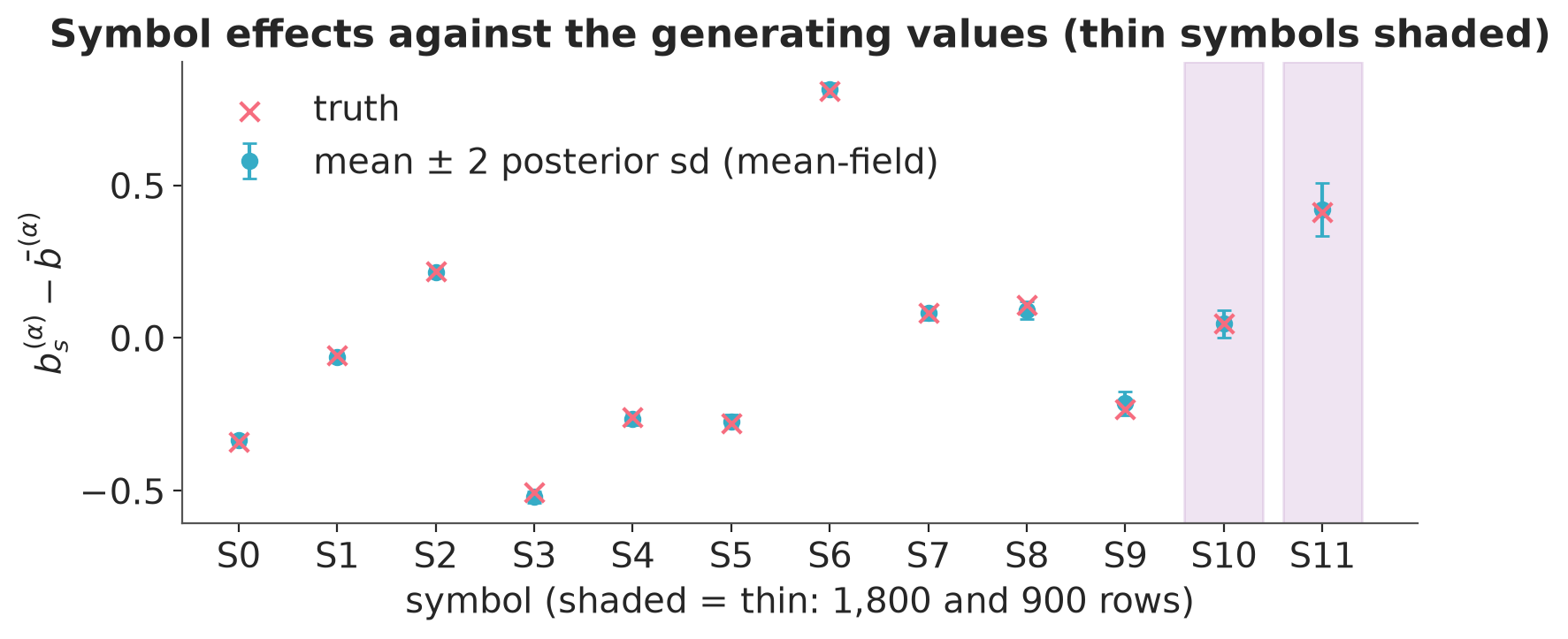
The posterior spread is widest for the symbols with the least data (the printout orders them), which is the hierarchy expressing that it knows less about those groups [Gelman and Hill, 2006]. The point estimates track their generating values across the board, including the thin ones.

What the figure does not show is shrinkage in the strict sense: that would need an unpooled per-symbol fit to compare against, and this notebook does not run one. Nor are the bars calibrated intervals; the paragraph above declined to treat mean-field widths that way, and that applies to their ordering too. And whether pooling improves held-out prediction on real data is a separate question again, which nothing here tests.

What do those parameters mean as objects? For one symbol, holding the covariates at \(a = q = 0\), the fit implies two curves over the event clock: the probability that the next event leaves the price unchanged, and the 90% half-width of the move given that one happens. Both are built from global-plus-symbol sums, so neither sits on the translation ridge.

s_idx, hours = 0, np.arange(24)
Bh = hour_basis(hours)  # (24, 4)
# .dataset: idata.posterior is a DataTree in arviz 1.x
st = post.dataset.stack(sample=("chain", "draw"))


def pick(name, *dims):
    return st[name].transpose(*dims, "sample").values


logit_pi = (
    pick("kappa0")[None, :]
    + pick("b_k", "symbol")[s_idx][None, :]
    + Bh @ (pick("c", "harmonic") + pick("b_ph", "symbol", "harmonic")[s_idx])
)
log_sigma = (
    pick("alpha0")[None, :]
    + pick("b_al", "symbol")[s_idx][None, :]
    + Bh @ (pick("g", "harmonic") + pick("b_sh", "symbol", "harmonic")[s_idx])
)
# transform each draw, then summarize: the median of a function, not a function of medians
zero_prob = np.median(1.0 / (1.0 + np.exp(logit_pi)), axis=1)
half90 = np.median(np.exp(log_sigma) * stats.t.ppf(0.95, pick("nu"))[None, :], axis=1)

t_logit = (
    truth["kappa0"]
    + 0.30 * z_truth["z_k"][s_idx]
    + Bh @ (truth["c"] + 0.15 * z_truth["z_ph"][s_idx])
)
t_logsig = (
    truth["alpha0"]
    + 0.35 * z_truth["z_al"][s_idx]
    + Bh @ (truth["g"] + 0.12 * z_truth["z_sh"][s_idx])
)

fig, axs = plt.subplots(1, 2, figsize=(9, 3.2), layout="constrained")
for ax, post_curve, truth_curve, ylab in [
    (axs[0], zero_prob, 1.0 / (1.0 + np.exp(t_logit)), "P(next event does not move)"),
    (axs[1], half90, np.exp(t_logsig) * stats.t.ppf(0.95, truth["nu"]), "90% half-width (bp)"),
]:
    ax.plot(hours, post_curve, color="C0", lw=2, label="posterior median")
    ax.plot(hours, truth_curve, color="C1", ls="--", lw=1.5, label="generator truth")
    ax.set_xlabel("UTC hour")
    ax.set_ylabel(ylab)
axs[0].legend(fontsize=9)
fig.suptitle(f"SYM{s_idx:02d} on the event clock, at a = q = 0", fontsize=11);

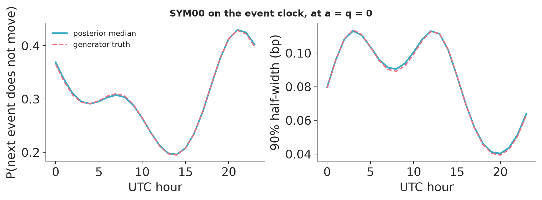
The half-width is a quantile of the outcome distribution, not a credible band for the curve: it answers “how far does a move go”, and it stays finite for any \(\nu > 0\). That is why the notebook reports it instead of a conditional standard deviation: the Student-t variance exists only for \(\nu > 2\), and nothing in this model guarantees that. Under this generator, the fit recovers both shapes; on real data the same two curves would be estimates, and would need out-of-sample evaluation before being used for anything.

In-sample posterior predictive adequacy

A recovery table checks parameters; a posterior predictive check asks the model to reproduce the data features it exists to describe. The CustomDist carries a random implementation alongside its logp, so sample_posterior_predictive() works out of the box. The two features that matter for this model are the exact-zero share and the heavy conditional tail; the figure after the table shows the whole empirical cumulative distribution function (ECDF) of one batch against sixty predictive draws:

eval_batch = next(iter(loader))
model["batch"].set_value(eval_batch, borrow=True)  # same path the callback uses
with model:
    idata = pm.sample_posterior_predictive(
        idata,
        var_names=["y_obs"],
        random_seed=RANDOM_SEED,
        extend_inferencedata=True,
        progressbar=False,
    )

pp = idata.posterior_predictive["y_obs"].stack(sample=("chain", "draw")).values.T
y_eval = eval_batch[:, 0]

zero_share = (pp == 0).mean(axis=1)
med_nonzero = np.array([np.median(np.abs(d[d != 0])) for d in pp[:500]])
q99_nonzero = np.array([np.quantile(np.abs(d[d != 0]), 0.99) for d in pp[:500]])


def check_row(observed, draws):
    lo, hi = np.quantile(draws, [0.05, 0.95])
    return [observed, draws.mean(), lo, hi]


y_nonzero = np.abs(y_eval[y_eval != 0])
pd.DataFrame(
    [
        check_row((y_eval == 0).mean(), zero_share),
        check_row(np.median(y_nonzero), med_nonzero),
        check_row(np.quantile(y_nonzero, 0.99), q99_nonzero),
    ],
    columns=["observed", "predictive mean", "predictive 5%", "predictive 95%"],
    index=["zero share", "median |move| (bp)", "q99 |move| (bp)"],
).round(3)

	observed	predictive mean	predictive 5%	predictive 95%
zero share	0.300	0.322	0.299	0.346
median |move| (bp)	0.039	0.040	0.037	0.043
q99 |move| (bp)	0.298	0.331	0.268	0.410

# hand-rolled ECDF: the bespoke feature is the annotated discrete jump at zero,
# which the predictive must reproduce in both location and height
fig, ax = plt.subplots(figsize=(8, 3.5), layout="constrained")
grid = np.linspace(-0.5, 0.5, 801)
for draw in pp[:60]:
    ax.plot(grid, np.searchsorted(np.sort(draw), grid) / draw.size, color="C0", alpha=0.08, lw=1)
ax.plot(
    grid, np.searchsorted(np.sort(y_eval), grid) / y_eval.size, color="k", lw=1.6, label="observed"
)
ax.plot([], [], color="C0", label="posterior predictive (60 draws)")
zero_jump = (y_eval == 0).mean()
below = (y_eval < 0).mean()
ax.annotate(
    f"vertical step at exactly 0:\nthe zero share ({zero_jump:.0%})",
    (0.03, below + zero_jump / 2),
    fontsize=9,
    ha="left",
    va="center",
)
ax.set_xlabel("next-event return (bp)")
ax.set_ylabel("empirical CDF")
ax.set_title("Posterior predictive ECDF: the step at zero is the hurdle")
ax.legend(loc="upper left");

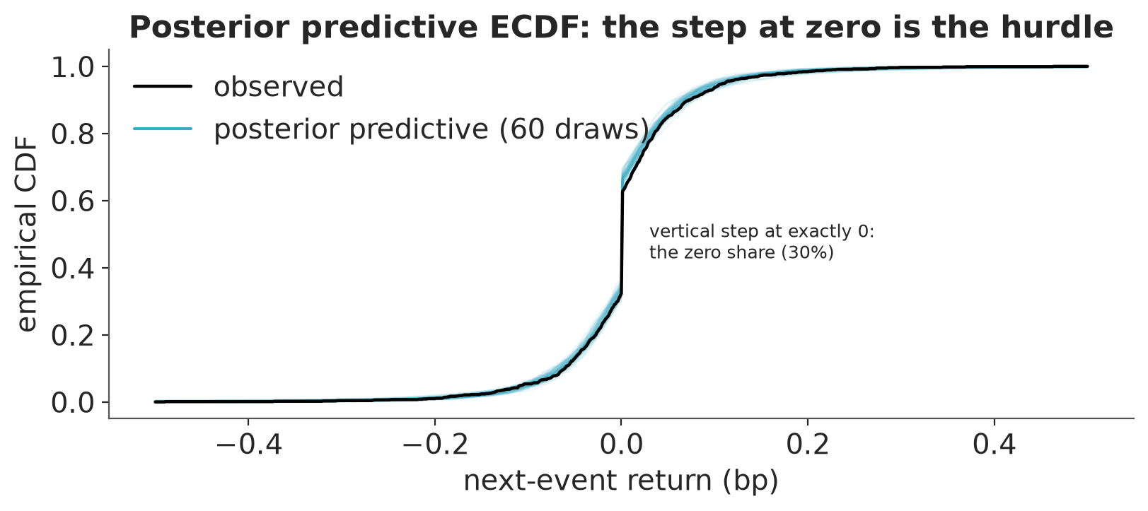
All three statistics sit inside their predictive 90% bands, though the zero share sits close to the lower edge, 0.300 observed against a band starting at 0.299, so it is a pass with almost no margin rather than a comfortable one. What that establishes is limited in two ways. The heading is literal: the evaluation batch was seen during the fit, so this is adequacy, not generalization, and a held-out split is the next thing to add before any of this is used to compare models. And the check is one batch, one step ahead, with the observed ylag held fixed: it does not simulate a price path forward, and it says nothing about the hierarchy, the hourly curves, or the covariate responses, each of which would need its own stratified check.

What a stopping rule has to be able to see

A streamed ELBO trace is noisy: every value is a one-batch, one-Monte Carlo estimate, so consecutive losses differ mostly because the batch changed. That makes “has it converged?” a signal-detection problem, and the horizon over which you look is the whole game.

Write the standardized block contrast at horizon \(w\): average the \(w\) losses before a point, average the \(w\) losses after it, and divide the difference by the noise scale of that difference,

\[ z_w(t) = \frac{\bar L_{t-2w:t-w} - \bar L_{t-w:t}} {\hat\sigma \sqrt{2/w}}, \]

with \(\hat\sigma\) estimated from successive differences. Positive \(z_w\) means the loss fell. For noise without long memory, averaging divides it by \(\sqrt{w}\) while a steady drift accumulates linearly in \(w\), so the detectable drift shrinks like \(w^{-3/2}\): the horizon does not merely smooth the picture, it sets what is visible at all. A fixed replay order is not noise of that kind, and the printout below shows where the generic scaling breaks, in the notebook’s favor.

# Stage 2 only, on the full-data scale: after the last planned optimizer change,
# which is where a stopping decision would actually be taken.
stage2 = loss[6_000:]
sigma_hat = np.mean(np.abs(np.diff(stage2))) * np.sqrt(np.pi) / 2.0


def signed_z(losses, w):
    """Standardised contrast between adjacent blocks of w losses."""
    csum = np.concatenate([[0.0], np.cumsum(losses)])
    t = np.arange(2 * w, len(losses))
    older = (csum[t - w] - csum[t - 2 * w]) / w
    newer = (csum[t] - csum[t - w]) / w
    return t, (older - newer) / (sigma_hat * np.sqrt(2.0 / w))


horizons = [(1, "per step"), (steps_per_epoch, "one epoch"), (2 * steps_per_epoch, "two epochs")]
# control: a horizon that is NOT a whole number of passes, to test whether the
# variance collapse below is really about epoch alignment
control = [(steps_per_epoch + steps_per_epoch // 2, "1.5 epochs")]
spreads = {}
for w, label in horizons + control:
    _, z = signed_z(stage2, w)
    spreads[label] = z.std()
    print(
        f"{label:>10s} (w={w:4d}):  mean z {z.mean():+.3f}   sd {z.std():.2f}"
        f"   |mean|/sd {abs(z.mean()) / z.std():.2f}"
    )
aligned = max(spreads["one epoch"], spreads["two epochs"])
print(f"\ncontrol spread is {spreads['1.5 epochs'] / aligned:.0f}x the widest aligned spread")

  per step (w=   1):  mean z -0.001   sd 0.99   |mean|/sd 0.00
 one epoch (w= 300):  mean z +0.014   sd 0.03   |mean|/sd 0.56
two epochs (w= 600):  mean z +0.034   sd 0.02   |mean|/sd 2.06
1.5 epochs (w= 450):  mean z +0.021   sd 0.45   |mean|/sd 0.05

control spread is 18x the widest aligned spread

fig, (ax, ax_zoom) = plt.subplots(
    1, 2, figsize=(9, 3.2), layout="constrained", gridspec_kw={"width_ratios": [3, 2]}
)
for (w, label), color in zip(horizons, ["C7", "C0", "C1"]):
    t, z = signed_z(stage2, w)
    ax.plot(
        t,
        z,
        color=color,
        lw=0.9 if w == 1 else 1.6,
        alpha=0.5 if w == 1 else 1.0,
        label=f"{label} (w={w})",
    )
    if w > 1:
        ax_zoom.plot(t, z, color=color, lw=1.6, label=f"{label} (w={w})")
for ax_ in (ax, ax_zoom):
    ax_.axhline(0.0, color="k", lw=0.8)
    ax_.set_xlabel("step within stage 2")
ax.set_ylabel(r"block contrast $z_w$")
ax.set_title("Same trace, three horizons", fontsize=11)
ax.legend(fontsize=8, loc="upper right", frameon=True)
ax_zoom.set_ylim(-0.12, 0.12)
ax_zoom.set_title(
    f"Aligned horizons only (control sd {spreads['1.5 epochs']:.2f} would fill this)", fontsize=10
)
ax_zoom.legend(fontsize=8, loc="upper right", frameon=True);

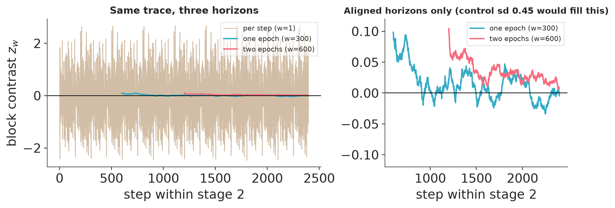
Read the printout as three signal-to-noise ratios, and the figure as the same thing twice: the left panel puts all three horizons on one scale, the right panel zooms in on the two that are invisible at that scale. At \(w = 1\) the standardized contrast has unit spread (which is what the \(\sqrt{2/w}\) scaling is built to produce) and a mean indistinguishable from zero: a single increment says nothing about the trend.

At the two epoch-aligned horizons the spread collapses far below what independent noise would predict, and the control row explains why. The shuffle is done once on disk and replayed in the same order every epoch, so a window of exactly one or two passes averages over the same rows every time and the batch-composition noise, which dominates the per-step view, all but drops out. Widen the window to one and a half passes and it does not: the printed ratio puts the control an order of magnitude above the wider of its two neighbors, even though it is itself wider than the one-epoch window. Nothing but the alignment changed.

What survives is Monte Carlo noise and the parameter drift itself, and against that much smaller yardstick the drift becomes visible: the ratio in the last column rises with the horizon. So, with a fixed replay order, the useful horizons are the ones commensurate with an epoch. That is a property of how the data was shuffled, not of the optimizer.

Why a naive rule fires instead of staying silent

It is tempting to accumulate per-step evidence with a one-sided cumulative-sum statistic of the kind Page [1954] introduced, here adapted to the standardized improvement: \(S \leftarrow \max(0,\ S + (\kappa - \max(z, 0)))\), stopping when \(S\) exceeds a threshold. Read carefully, that recursion behaves sensibly while there is signal: if the standardized improvement stays above \(\kappa\), the increment is negative and \(S\) sits at zero. The difficulty is what happens when there is no resolvable signal. Under symmetric noise \(\mathbb{E}[\max(z,0)]\) is only a fraction of a standard deviation, so with \(\kappa\) above that value \(S\) climbs at a roughly constant rate and crosses any fixed threshold after a roughly fixed number of steps. The rule therefore cannot tell “converged” from “still improving, but too slowly for this horizon to see”; it announces the same thing at the same pace in both cases. So the fix is not a better threshold but a wider horizon, plus a second yardstick that asks whether the remaining improvement is negligible relative to the reduction already achieved. That design is implemented in pymc-extras#733; this notebook shows the observation problem it exists to solve rather than shipping a second copy of it.

How much would an online rule be worth here? The retrospective answer is a benchmark you can only compute afterwards, which is why the online version is needed:

# t99: the first step at which a trailing average of width one epoch has covered
# 99% of stage 2's total smoothed reduction. Retrospective by construction.
kernel = np.ones(steps_per_epoch) / steps_per_epoch
smoothed = np.convolve(stage2, kernel, mode="valid")
total_drop = smoothed[0] - smoothed.min()
# "valid" convolution starts at the first full window, so index j of `smoothed`
# is the trailing average ending at stage-2 step j + steps_per_epoch, counting
# steps from 1.
t99 = int(np.argmax(smoothed <= smoothed.min() + 0.01 * total_drop)) + steps_per_epoch
print(
    f"stage 2 smoothed reduction: {total_drop:,.2f} nats;\n"
    f"99% of it reached by step {t99:,} of {len(stage2):,} "
    f"({t99 / len(stage2):.0%} of the stage-2 budget)"
)

stage 2 smoothed reduction: 188.11 nats;
99% of it reached by step 1,947 of 2,400 (81% of the stage-2 budget)

Any stopping rule, this one included, comes with two qualifications. What such a rule detects is a loss plateau, a necessary signal, not a proof that the posterior has converged; the recovery and predictive checks above are the kind of independent evidence a stop should be paired with. And a plateau in a noisy loss can only ever be established relative to a horizon: at any finite step, an improvement small enough is indistinguishable from none.

Related tooling in pymc-extras

The loader used above is one of four streaming pieces in pymc-extras. The others are not imported here; this is where each one fits.

Component	What it does
DataLoader / parquet_source	Turns an out-of-core source into minibatches and owns total_size; used directly above
Trainer	Wraps the data-advance lifecycle around pm.fit, the job the twenty-line StreamAdvance does here
CheckLossConvergence	Loss-based stopping on growing block horizons with two yardsticks; the observation problem it addresses is the previous section
streaming Pathfinder	A short quasi-Newton run on minibatch gradients that returns a Gaussian proposal, importance-corrected against the full-data log-density, with Pareto-\(k\) as its own veto

Pathfinder is the faster route when an approximately placed starting point is what you need, for example to initialize Markov chain Monte Carlo (MCMC). It is not run here, and the reason is a decision taken before fitting rather than a result: its documented operating range is non-hierarchical targets of at most a few tens of parameters, and this target is hierarchical with

n_free = DictToArrayBijection.map(model.initial_point()).data.size
print(f"free parameters in the unconstrained space: {n_free}")

free parameters in the unconstrained space: 154

free parameters, an order of magnitude outside that range. The ADVI results above stand or fall on their own recovery and predictive checks, independently of this choice.

Acknowledgements

This notebook was written as part of the 2026 Google Summer of Code project Streaming Variational Inference for Large Datasets with PyMC and NumFOCUS, mentored by Rob Zinkov and Chris Fonnesbeck.

Authors

• Authored by Yicheng Yang in August 2026 (pymc-examples#892)

References

[1] (1,2)

Andrew Gelman and Jennifer Hill. Data analysis using regression and multilevel/hierarchical models. Cambridge University Press, 2006. doi:10.1017/CBO9780511790942.

[2]

Alp Kucukelbir, Rajesh Ranganath, Andrew Gelman, and David M. Blei. Automatic variational inference in stan. 2015. arXiv:1506.03431.

[3]

Matthew D. Hoffman, David M. Blei, Chong Wang, and John Paisley. Stochastic variational inference. Journal of Machine Learning Research, 14:1303–1347, 2013. URL: https://jmlr.org/papers/v14/hoffman13a.html.

[4]

Robert F. Engle and Jeffrey R. Russell. Autoregressive conditional duration: a new model for irregularly spaced transaction data. Econometrica, 66(5):1127–1162, 1998. doi:10.2307/2999632.

[5]

Torben G. Andersen and Tim Bollerslev. Intraday periodicity and volatility persistence in financial markets. Journal of Empirical Finance, 4(2-3):115–158, 1997. doi:10.1016/s0927-5398(97)00004-2.

[6]

Tim Bollerslev. A conditionally heteroskedastic time series model for speculative prices and rates of return. The Review of Economics and Statistics, 69(3):542–547, 1987. doi:10.2307/1925546.

[7]

Richard Roll. A simple implicit measure of the effective bid-ask spread in an efficient market. The Journal of Finance, 39(4):1127–1139, 1984. doi:10.1111/j.1540-6261.1984.tb03897.x.

[8]

Boris T. Polyak and Anatoli B. Juditsky. Acceleration of stochastic approximation by averaging. SIAM Journal on Control and Optimization, 30(4):838–855, 1992. doi:10.1137/0330046.

[9]

E. S. Page. Continuous inspection schemes. Biometrika, 41(1-2):100–115, 1954. doi:10.1093/biomet/41.1-2.100.

Watermark

%load_ext watermark
print(f"wall time for every cell above, on this machine: {time.perf_counter() - NOTEBOOK_T0:.0f} s")
%watermark -n -u -v -iv -w -p xarray
%watermark -m

wall time for every cell above, on this machine: 42 s
Last updated: Tue, 18 Aug 2026

Python implementation: CPython
Python version       : 3.12.12
IPython version      : 9.16.1

xarray: 2026.7.0

arviz      : 1.3.0
logging    : 0.5.1.2
matplotlib : 3.11.1
numpy      : 2.4.6
pandas     : 3.0.5
pyarrow    : 25.0.1
pymc       : 6.2.0
pymc_extras: 0.14.1.dev3+g8db1880d4
pytensor   : 3.2.4
scipy      : 1.18.0

Watermark: 2.6.0

Compiler    : Clang 21.1.4 
OS          : Darwin
Release     : 24.6.0
Machine     : arm64
Processor   : arm
CPU cores   : 10
Architecture: 64bit

License notice

All the notebooks in this example gallery are provided under the MIT License which allows modification, and redistribution for any use provided the copyright and license notices are preserved.

Citing PyMC examples

To cite this notebook, use the DOI provided by Zenodo for the pymc-examples repository.

Important

Many notebooks are adapted from other sources: blogs, books… In such cases you should cite the original source as well.

Also remember to cite the relevant libraries used by your code.

Here is an citation template in bibtex:

@incollection{citekey,
  author    = "<notebook authors, see above>",
  title     = "<notebook title>",
  editor    = "PyMC Team",
  booktitle = "PyMC examples",
  doi       = "10.5281/zenodo.5654871"
}

which once rendered could look like: